For an introduction to stable diffusion, have a look at an earlier post were the main components are described.
Diffusion process
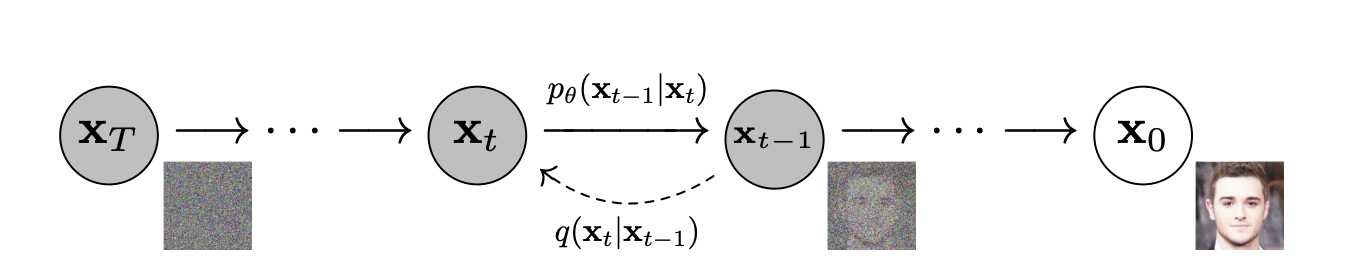
Diffusion is a technique for generating new images that resemble the data distribution: the distribution of images that the model was trained on. It does this by making use of a diffusion process, which can be visualized with the diagram below. In the diagram on the right, \(x_0\) represents a clean image without any noise. On the left, \(x_T\) represents an image that is pure noise. The variable \(x\) thus represents a high dimensional tensor where the amount of dimensions is equal to the amount of pixels.
In between these, we see a number of intermediate states \(x_t\) which represent images that are a mix of the clean and the pure noise image. We can transition from state to state with \(p_\theta\) and \(q\).
More precisely, \(q\) represents the forward diffusion process. With \(q\) we can move to the left, i.e. we can move from images with less noise to images with more noise. Note that \(q(x_t|x_{t-1})\) shows that it’s a probability distribution, it’s not a deterministic function that always returns a fixed image \(x_t\) for the same \(x_{t-1}\). Instead it defines a probability distribution over all possible images \(x_t\).
Diffusion processs
Similarly, we have a probability distribution \(p_\theta(x_{t-1}|x_t)\) which we can use to move to the right. From an image with some noise, we can sample an image from this distribution that has less noise. This is called the reverse process.
To be able to generate new images according to the data distribition we thus need an expression for the reverse process so that we can iteratively remove the noise from a pure noise image \(x_T\).
Stochastic perspective
For a deterministic function we write \(y = f(x)\) to represent that \(y\) is some function of \(x\). It’s deterministic in the sense that calling the same value of \(x\) multiple times on \(f\), will always returns the same value of \(y\). In this setting we are generally interested in finding the function \(f\). So that for any unseen \(x\), we can have a prediction for \(y\). For stochastic systems (which are considered in stable diffusion), we are dealing with random variables Y and X, and there doesn’t exist a deterministic function \(f\). Instead we are interested in finding the probability density function \(p(Y=y | X=x) = p(y|x)\) which represents the probability that random variable Y takes on value y, given that random variable X takes on value x, which is the stochastic equivalent of \(f\). With \(p(y|x)\), we have (an estimate) of all the possible values \(y\) can take on and the associated probabilities, given some input \(x\). This means we can sample from this distribution, to get realistic \(y\) values given some value of \(x\).
What helps me to think in this stochastic perspective for high dimensional images, is to simply think of 1 dimensional variables weight (\(Y\)) and height (\(X\)) of a person:
Realize that these are random variables, different people have different weights and heights.
There is a relation between the two: people that are taller are generally more heavy. In other words: if you have to make a guess for a person’s weight, you would probably make a better guess if I tell you the height of this person.
The relation between weight and height is not deterministic. Not every person with the same height has the same weight. Consequently, knowing the height of the person gives us at best the possible weight values and the probabilities (the probability density function \(p(y|x)\)).
Once \(p(y|x)\) has been determined, we can sample a realistic value of a person’s weight, given it’s height.
Noise and the forward process
The forward process is very straight forward, we simply take our current image and add some noise to it. The noise (denoted by \(\epsilon\)) being a tensor with the same shape as the image which values are sampled from some distribution, for example the standard normal distribution\(\mathcal{N}(\epsilon;0,1)\). Below two noise images are displayed, on the left an black-and-white image (1 channel), on the right a 3 channel RGB image.
# Code taken from to help with plotting:# https://github.com/fastai/course22p2/blob/df9323235bc395b5c2f58a3d08b83761947b9b93/nbs/05_datasets.ipynbdef subplots( nrows=1, # Number of rows in returned axes grid ncols=1, # Number of columns in returned axes grid figsize=None, # Width, height in inches of the returned figure imsize=3, # Size (in inches) of images that will be displayed in the returned figure suptitle=None, # Title to be set to returned figure**kwargs): # fig and axs"A figure and set of subplots to display images of `imsize` inches"if figsize isNone: figsize=(ncols*imsize, nrows*imsize) fig,ax = plt.subplots(nrows, ncols, figsize=figsize, **kwargs)if suptitle isnotNone: fig.suptitle(suptitle)if nrows*ncols==1: ax = np.array([ax])return fig,axdef get_grid( n, # Number of axes nrows=None, # Number of rows, defaulting to `int(math.sqrt(n))` ncols=None, # Number of columns, defaulting to `ceil(n/rows)` title=None, # If passed, title set to the figure weight='bold', # Title font weight size=14, # Title font size**kwargs,): # fig and axs"Return a grid of `n` axes, `rows` by `cols`"if nrows: ncols = ncols orint(np.floor(n/nrows))elif ncols: nrows = nrows orint(np.ceil(n/ncols))else: nrows =int(math.sqrt(n)) ncols =int(np.floor(n/nrows)) fig,axs = subplots(nrows, ncols, **kwargs)for i inrange(n, nrows*ncols): axs.flat[i].set_axis_off()if title isnotNone: fig.suptitle(title, weight=weight, size=size)return fig,axsdef show_image(im, ax=None, figsize=None, title=None, noframe=True, **kwargs):"Show a PIL or PyTorch image on `ax`."if fc.hasattrs(im, ('cpu','permute','detach')): im = im.detach().cpu()iflen(im.shape)==3and im.shape[0]<5: im=im.permute(1,2,0)elifnotisinstance(im,np.ndarray): im=np.array(im)if im.shape[-1]==1: im=im[...,0]if ax isNone: _,ax = plt.subplots(figsize=figsize) ax.imshow(im, **kwargs)if title isnotNone: ax.set_title(title) ax.set_xticks([]) ax.set_yticks([]) if noframe: ax.axis('off')return axdef show_images(ims, # Images to show nrows=None, # Number of rows in grid ncols=None, # Number of columns in grid (auto-calculated if None) titles=None, # Optional list of titles for each image**kwargs):"Show all images `ims` as subplots with `rows` using `titles`" axs = get_grid(len(ims), nrows, ncols, **kwargs)[1].flatfor im,t,ax in zip_longest(ims, titles or [], axs): show_image(im, ax=ax, title=t)
bw_noise = torch.randn(64, 64) # 1 channel: Black and whitergb_noise = torch.randn(64, 64, 3) # 3 channels: RGBfig, axs = plt.subplots(1, 2, figsize=(10,5))axs[0].imshow(bw_noise.clamp(0,1));axs[1].imshow(rgb_noise.clamp(0,1));axs[0].set_title("Black and White Noise")axs[1].set_title("RGB Noise")axs[0].axis('off');axs[1].axis('off');
Let’s see what happens when we iteratively add more and more noise to an image:
im = Image.open('./image.png')im = (torchvision.transforms.functional.pil_to_tensor(im) /255.0).permute(1,2,0)shape = im.shapeplots =5fig, axs = plt.subplots(1, plots, figsize=(15,10));axs[0].imshow(im);axs[0].axis('off');for i inrange(1,plots): noise = torch.randn(shape) *0.5 im = (im + noise).clip(0,1) axs[i].imshow(im); axs[i].axis('off')
On the left, we start with a clean image, and gradually add more and more noise to it. Diffusion based models are defined as models in which the forward (or diffusion, noising) process is fixed to a Markov chain that gradually adds Gaussian noise to the data according to a variance schedule. A Markov chain is simply a (stochastic) process with a fixed number of states and transition probabilities that only depend on the current state, and are therefore memoryless. This forward process is defined as:
The forward process is indeed memoryless, since the probability distribution over \(x_t\) only depends on \(x_{t-1}\) and not any earlier state. The probability distribution in question is a normal distribution (\(\mathcal{N}\)) centered around \(\mu = \sqrt{1-\beta_t}x_{t-1}\) with a variance of \(\beta_t I\). \(\beta_t\) is called the variance schedule and is simply a constant that only depends on \(t\). The identity matrix \(I\) reflects that there is no dependency (for the random component) between the different pixels. The authors in the paper run experiments with \(T=1000\) (fixed number of states: the second condition that makes this a Markov chain) and a fixed variance schedule running from \(\beta_1 = 10^{-4}\) to \(\beta_T = 0.02\). Let’s define this in code:
T =1000beta = torch.linspace(1e-4, 1e-2, T)
plt.plot(beta);
So we have a linear variance schedule, starting on the left with T=1 and a very small value for \(\beta\) and then increasing linearly to larger values.
Furthermore, we can re-write the forward process in a way that allows to express \(q\) in terms of the clean image \(x_0\):
where \(\alpha_t = 1-\beta_t\) and \(\bar\alpha_t = \prod_{s=1}^t \alpha_s\). This allows to immediately compute some intermediate image \(x_t\) from the clean image \(x_0\), without doing all the intermediate steps. Let’s also put this into code:
From the figure on the right for \(\bar\alpha_t\), we see an interesting property: the value for \(t=1\) is almost 1, and the last value (\(t=999\)) goes towards 0. Plugging these values into the normal distribution above, we see that \(x_1\) is centered almost exactly at \(x_0\) and has very little noise, whereas \(x_{999}\) is centered around 0 and has (almost) unit variance noise. We thus indeed diffuse from a clean image into an image consisting purely of (standard normal) noise.
To understand how we can create (samples from) the forward process, we have to understand how we can create samples from the normal distribution defined above. For that purpose it’s intructive to review some basic arithmetic rules around random variables. Let’s say \(X = \mathcal{N}(0,1)\) and \(Y = 5X + 3\), then \(Y\) is also going to be normally distributed, but the mean and variance will have shifted, let’s see how:
Then, to get a normal distribition: \(\mathcal{N}(x_t; \sqrt{\bar\alpha_t}x_0, (1-\bar\alpha_t)I)\), we can thus sample from a standard normal distribution and simply add the mean: \(\sqrt{\bar\alpha_t}x_0\) (\(x_0\) being the clean image) and multiply by: \(\sqrt{1-\bar\alpha_t}\) (note the usage of the square root to cancel out the squaring of the constant). Let’s do this in code:
im = Image.open('./image.png')im = (torchvision.transforms.functional.pil_to_tensor(im) /255.0).permute(1,2,0)plots =5fig, axs = plt.subplots(1, plots, figsize=(15,10));axs[0].imshow(im);axs[0].axis('off');ts = np.linspace(0, T-1, plots)for i inrange(0,plots): t =int(ts[i]) alpha_bar_t = alpha_bar[t]# take a sample from N(0,1) noise = torch.randn(shape)# move the sample to the specified mean and variance im = (np.sqrt(alpha_bar_t)*im + np.sqrt((1-alpha_bar_t))*noise).clip(0,1) axs[i].imshow(im); axs[i].axis('off') axs[i].set_title(f't = {t}')
These images are actual samples from the forward diffusion process as specified by the DDPM paper. Note that already from t=499 onward it’s practically impossible to see what the clean image was depicting. We will see this again later on.
Reverse process
Now that we have a good understanding of the concepts, the notation and the forward process, let’s continue with the reverse process. This reverse process is what we are actually interested in, since it allows us to generate images from pure noise. But before we do, take a moment to realize how difficult this actually is. Imagine the very high dimensional pixel space, where each pixel is a separate dimension. For a 128 by 128 image (a small image), that is more than 16000 dimensions. Any position in this space represents an image, but if we randomly select any position in this space the chances are extremely small that we will pick an image that depicts anything different from noise. This means that the data distribution is very small in comparison to this space, and to compute a path from any random point to this data distribution is not trivial.
In the paper, the reverse process is described as follows:
So to take one step to the right we need to sample from a distribution with mean \(\mu_\theta\) and variance \(\Sigma_\theta\). These two expressions are unknown, and thus will have to be learned by a neural network (as represented by the \(\theta\) subscript, denoting the parameters of the network). The authors decide to disregard the \(\Sigma_\theta\) network because it leads to unstable training and poorer sample quality. Instead it’s set to a time dependant constant: \(\sigma_t^2 = \beta_t\) or \(\sigma_t^2 = \tilde\beta_t = \frac{1-\bar\alpha_{t-1}}{1-\bar\alpha_t}\beta_t\).
This means, we are left with one neural network \(\mu_\theta(x_t, t)\) which has to be trained for the mean of the normal distribution. In the paper it is shown by using maximum likelihood estimation, variational inference, evidence lower bound, KL divergence and reparametrizations, that a simplified loss function can be written as:
Which is arguably still quite a complex expression, so let’s digest it step by step.
On the left we have a loss function \(L_{\textrm{simple}}\) which is a function of \(\theta\). Denoting that the loss function is a function of all the parameters \(\theta\) of some neural network. In other words, we want to minimize the loss function by tweaking the parameters \(\theta\) in the neural network.
On the right side of the equation we have an expected value symbol \(\mathbb{E}[.]\), which we recognize to be similar to \(\mathbb{E} \left( \epsilon - \bar\epsilon \right)^2\) being the Mean Squared Error (MSE) of the estimator \(\bar\epsilon\) of parameter \(\epsilon\). The parameter \(\epsilon\) is defined in the paper to be the noise, and is simply sampled from a standard normal distribution.
The \(\epsilon_{\theta}\) symbol represents a neural network (again parametrised by it’s parameters \(\theta\)) estimating the noise (\(\epsilon\)). This network has two inputs: \(\sqrt{\bar\alpha_t} x_0 + \sqrt{1-\bar\alpha_t}\epsilon\) and \(t\). This first expression is simply a sampled noisy image originating from applying the forward process on some clean image \(x_0\) to timestep \(t\):
To summarize: \(\epsilon_{\theta}\) represents a neural network which predicts the noise in noisified images as computed by the forward process. We can create training data by using the formula for the forward process, and we will use an MSE loss on the predictions and the actual noise.
It’s also instructive to compare this to the pseudo-code describing the training of the neural network in the DDPM paper:
pseudo code for training
On the second line we simply take a clean image \(x_0\). Next, we randomly select a value for \(t\). Then we sample some noise from a standard normal distribution. On line 5, we do the forward pass on the noisy image, compute the MSE loss on the prediction and the actual loss, compute the backward pass and finally update the weights of our network.
Training: preparing the data
Let’s use the same data we have been using before: fashion-mnist:
Code
from datasets import load_dataset,load_dataset_builderfrom nntrain.dataloaders import DataLoaders, hf_ds_collate_fnfrom nntrain.learner import*from nntrain.activations import*import torchvision.transforms.functional as TFimport torchimport torch.nn as nnimport torch.nn.functional as Ffrom operator import attrgetterfrom functools import partialimport fastcore.allas fcimport mathimport torcheval.metrics as temimport matplotlib.pyplot as pltimport randomimport numpy as np
name ="fashion_mnist"ds_builder = load_dataset_builder(name)hf_dd = load_dataset(name)# Transform the images to 32x32 (from 28x28) so that the# convolutional arithmetic in the UNet worksdef transformi(b): b['image'] = [TF.resize(TF.to_tensor(o), (32,32)) for o in b['image']]return bhf_dd = hf_dd.with_transform(transformi)
Previously we created a custom collate function to pull the data out of the Huggingface DatasetDict object and put it in a tuple. For the purpose of a diffusion model, we need to change this collation function to make sure the DataLoader will return samples consisting of the noisy image \(q(x_t|x_0)\), the sampled timestep \(t\) and the noise \(\epsilon\). The noisy image and timestep \(t\) will be inserted into the model, and the noise \(\epsilon\) will be used as target for the MSE loss function.
To do this, let’s create a noisify function that returns everything we need:
def noisify(clean_images): N = clean_images.shape[0] t = torch.randint(low=0,high=T,size=(N,)) alpha_bar_t = alpha_bar[t, None, None, None] # add empty dimensions for broadcasting noise = torch.randn(clean_images.shape)# According to the forward process in the paper: noised_images = (alpha_bar_t.sqrt()*clean_images + (1-alpha_bar_t).sqrt()*noise)return noised_images, t, noise
Next, we are going to need a model. Remember that our model is going to take (noisy) images as input, and will also output images that represent predictions of the noise. One model that is capable of doing so, is a UNet. This model was shortly discussed in an earlier post. Let’s use a Unet model from the diffusers library:
model = UNet2DModel(in_channels=1,
                    out_channels=1,
                    block_out_channels=(16,32,64,64),
                    norm_num_groups=8)
Training
We need to make some changes to our Learner, to accomodate for the specific model we are using, and the fact that we are having items in the batch (noised image, timestep \(t\) and actual noise). Specifically, we need to overwrite the predict method:
We need to pass the first two items from the batch (noised image and timestep \(t\)) to the model
The Unet model we are using, is wrapping the result of the forward pass in a dictionary (with key sample), we thus need to pull this value out of the dictionary.
We also need to update the loss method, since the targets are stored as third item in the batch:
class DDPMLearner(Learner):def predict(self):self.preds =self.model(self.batch[0], self.batch[1]).sampledef get_loss(self): self.loss =self.loss_fn(self.preds, self.batch[2])
With the data, the model and the adapted training loop, we can now train as usual:
As a final step, we want to sample some images: we start with images of pure noise and by gradually removing the noise, we will hopefuly obtain clean images. In the paper, the following algorithm is presented:
pseudo code for sampling
On line 1, we start with a pure noise image \(x_T\). Next, we iterate through the timesteps (in reverse). During each step, a prediction of the noise in the image \(\epsilon_{\theta}(x_t, t)\) is made. Note that this is an estimate of all the noise in the image, e.g. the difference betweeen the seen image and the clean image. One could think that we thus could remove this noise from the image, and arrive immediately at a clean image. However, this is not what is done. Instead the scaled prediction is subtracted from the image (line 4), and some new (scaled) random noise \(z\) is added back. This added noise is less then what we removed, the idea being that the output \(x_{t-1}\) is a bit less noisy then the previous image \(x_t\).
That doesn’t look bad at all, especially considering that we are only training for 5 epochs. Comparing it to actual images from the training set below, we see that they are not quite as good, but we still can easily recognize the categories from the images and there is quite some detail in the images.
Let’s also have a look at an animation of the reverse process: starting from pure noise \(x_T\) and moving toward \(x_0\). It’s interesting to notice that in the majority of timesteps, the images look like pure noise and only in the last few hundred steps some structure is becoming visible. This hints at the idea, that there are probably improvements to be made to the noise schedule and the amount of steps, to more quickly arrive at \(x_0\) and as it turns out, many of the follow-up papers focus on this.
%matplotlib autoimport matplotlib.animation as animation from IPython.display import display, HTMLfig, ax = plt.subplots(figsize=(8,2))fig.tight_layout()ax.axis('off')ims = []for t, images inenumerate(preds): im = ax.imshow(torch.concat([i for i in images], dim=2).permute(1,2,0), animated=True) ims.append([im])ani = animation.ArtistAnimation(fig, ims, interval=10, blit=True, repeat_delay=50000)display(HTML(ani.to_html5_video()))